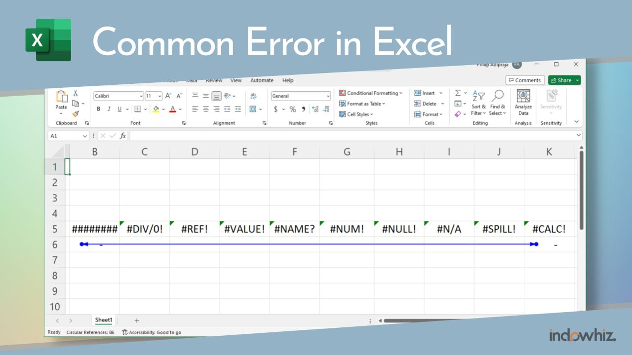
You may often see errors in Microsoft Excel, such as #####, #DIV/0!, #REF!, #VALUE!, #NAME?, #NUM!, #NULL, #N/A, #SPILL!, #CALC!, and Circular reference error. These errors indicate different kinds of problems with the formulas, references, or values in your worksheet. We’re here to help you find out why this happens and how to fix it.
1. ####
When you enter a value or a formula in a cell, Excel may display #### instead of the actual result. Fortunately, it is only a display issue. It shows #### when the cell is not wide enough to display the value or the result of a formula.
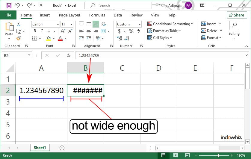
#### display issue in Excel because the column is not wide enough.There are several ways to fix this issue:
- Adjust column width.
To increase the column width, you can drag the right border of the column header or use theAutoFitfeature. - Change the number format.
If possible, you can change a value to a different format. You can use theFormat Cellsdialog box or theNumbergroup on theHometab. For example, you can reduce the number of decimal places or use scientific notation (like0.0E+00) to make the value fit in the cell. Or, use ashort dateformat rather than along dateformat. - Rotate the Text.
Another option is to rotate the text in the cell by an angle to make it fit in a narrow column. For example, you can use a45°or90°angle to display the text. You can change theOrientationon theHometab.
2. #DIV/0!
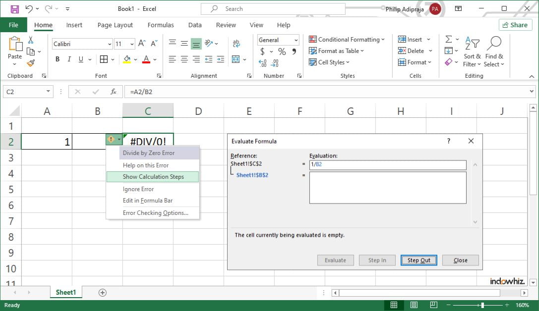
Well, the error message pretty much explains all of it. Excel displays it when a formula tries to divide a number by zero or by a blank cell. For example, if you enter “=5/0” or “=5/B2” where the B2 cell is blank.
Some of you may know that your formula is correct, and realize that #DIV/0! errors may occur. In this case, there are several things you can choose:
- Leave it as it is.
You know and don’t care about it. Then, you can leave it as is. - Changing error display.
Instead of#DIV/0!errors, you can alternatively change it into another error message, such as0, “Not Available“, or" "(blank).
There are several ways to achieve it. You can use eitherIFERROR,IF,ISERROR, orISERRfunction. However,IFERRORis the simplest one.
For example, if the formula that returns the error is=A2/B2, you can use=IFERROR(A2/B2, 0)to return0(zero)instead of the#DIV/0!error. You can change it using “Not Available“," "(blank), or any string you want.
However, if you expect that the divisor will not be zero, there are some ways to fix this error:
- Checking the divisor.
If you have a simple formula, you can directly check the value or reference cell of the divisor. Make sure that the divisor in your formula is not zero or blank. - Evaluate your formula to locate the source of error.
If you have a complex formula, you may useError Checkingfeature. You can access this feature by going to theFormulastab and clicking theError Checkingbutton. Or, you can click the button near the error cell. Then, click onShow Calculation Steps. Then, evaluate your formula step by step to find where and why you got zero divisor.
3. #REF!
Excel will show #REF! error, if a formula contains invalid or nonexistent references. Commonly, it happens when the cells or range that a formula refers to, were either nonexistent, moved, or deleted, as in Figure 3.
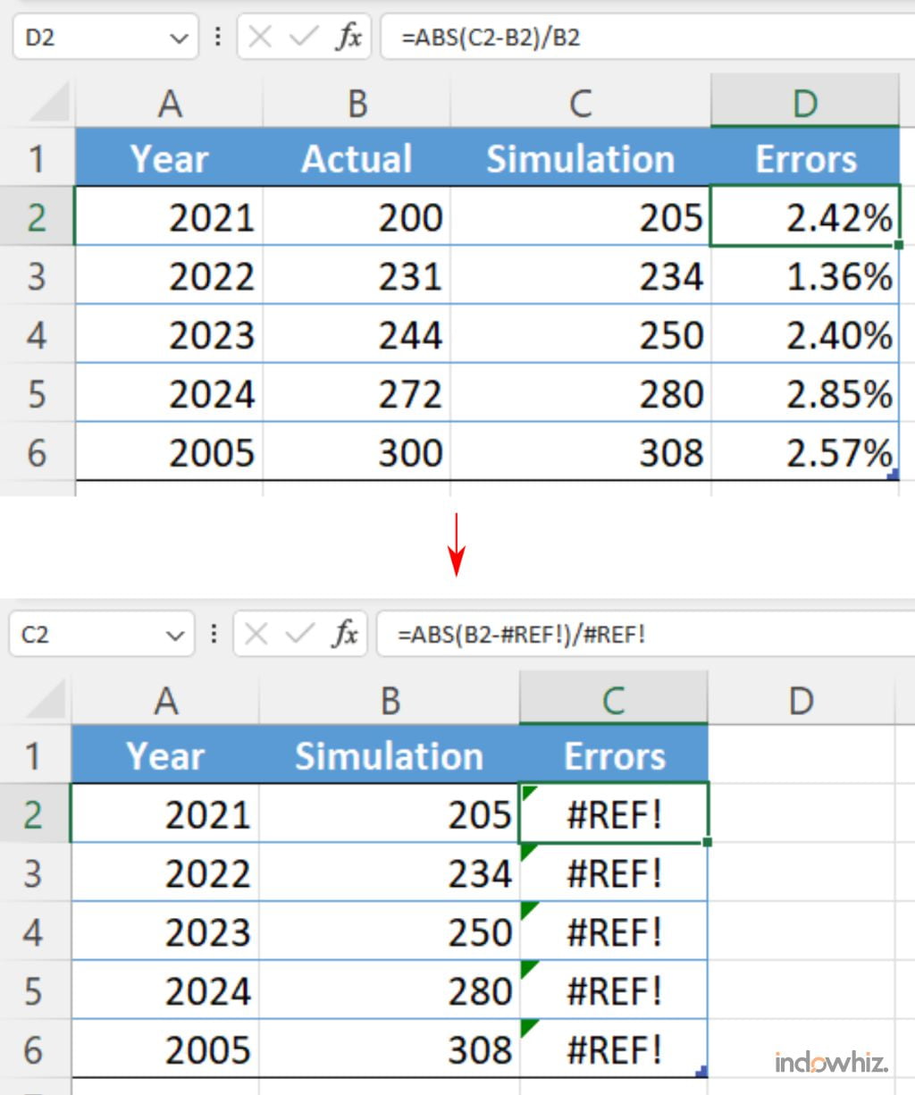
#REF! error due to deleted columnThere are different ways to find and fix #REF! error in Excel. Here are some of them:
- Undo the accidental move or delete actions.
If you accidentally move or delete the reference cells, range, columns, or rows, you can just undo your action (or pressCTRL+Z). - Evaluate your formula to locate the source of error.
If you have a complex formula, you may useError Checkingfeature. You can access this feature by going to theFormulastab and clicking theError Checkingbutton, or you can click the button near the error cell. Then, click onShow Calculation Steps. Then, evaluate your formula step by step to find where and why you got#REF!error.
For example, you may useVLOOKUPorINDEXfunction, in which you ask to return the value of the 4th column, but your reference range only has 3 columns. As a result, it will throw#REF!error. - Adjust the formula.
You may intend to move or delete the reference cells, which cause#REF!error. But, you can update the formula to reference the correct cells, range, columns, or rows.
4. #VALUE!
Excel shows #VALUE! error, when a formula includes any values that are incompatible with the function or operation used. For example, if you try to add two cell values and one of them contains text values, then the #VALUE! error will occur. It is not rare to find a space within a numeric value that makes its format becomes a text rather than a number, as illustrated in Figure 4.
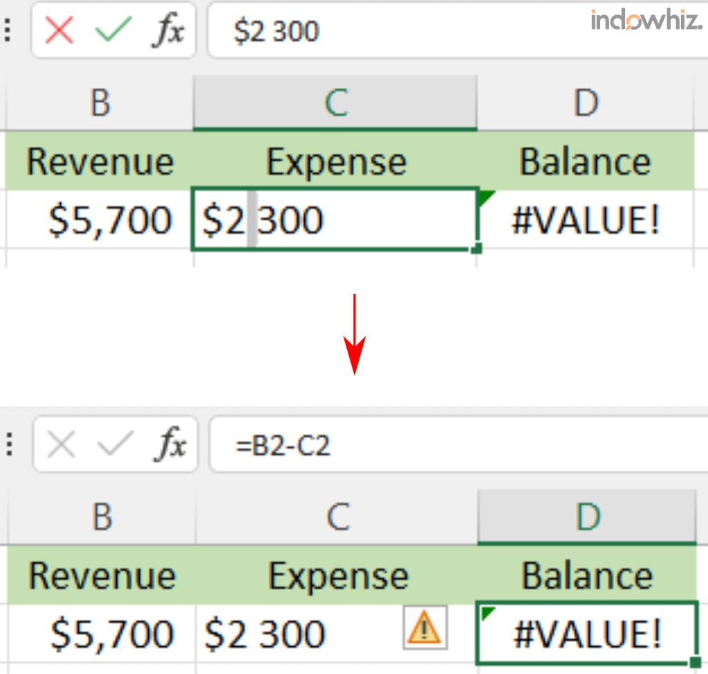
#VALUE! error due to space in the numeric valueSeveral ways you can choose to solve #VALUE! errors in Excel, such as:
- Evaluate your formula to locate the source of error.
If you have a complex formula, you may useError Checkingfeature. You can access this feature by going to theFormulastab and clicking theError Checkingbutton, or you can click the button near the error cell. Then, click onShow Calculation Steps. Then, evaluate your formula step by step to find where and why you got#VALUE!error. - Checking data types.
Make sure you use the correct data types in your function or operation. For example, if you useSUMorPRODUCTfunction, you need to use values or references to cells that contain numbers rather than text. - Removing spaces and special characters.
Make sure that there are no extra spaces or special characters in your formula or in the cells that you reference. For example, if you use a comma as a decimal separator, but your regional settings use a period as a decimal separator, you will get#VALUE!error. - Use another function.
Some functions or operations can only handle specific data types. Therefore, you may want to use another function that suits your needs. For example, instead of using “+” operator to combine values, you can use theCONCATENATEfunction to combine either number or text values.
5. #NAME?
The #NAME? is an error message that Excel displays when a formula contains an unrecognized name, such as:
- Misspelling.
For example, if you type=SUMM(A2:A6)instead of=SUM(A2:A6), Excel will not recognize the functionSUMMand return#NAME?error. - Incorrect cell reference.
For example, if you type=SUM(AB:A10)instead of=SUM(A2:A10), Excel will not be able to find the rangeAB:A10. - Misspelling a named range.
A named range is a group of cells that you can assign a descriptive name to and use in formulas instead of typing the cell references. For example, if you name the rangeA2:A6as Sales, you can use=SUM(Sales)instead of=SUM(A2:A6). However, if you misspell the name of the range or use it in a different worksheet than where it is defined, Excel will return a#NAME?error. - Missing or incorrect use of quotation marks for text values.
For example, if you type=VLOOKUP(Apple,A2:B6,2,FALSE)instead of=VLOOKUP(“Apple”,A2:B6,2,FALSE), Excel will think thatAppleis a named range or a function because did not use quotation marks (" ") and will return a#NAME?error.

#NAME?There are different ways to fix #NAME? errors in Excel, such as:
- Evaluate your formula to locate the source of error.
If you have a complex formula, you may useError Checkingfeature. You can access this feature by going to theFormulastab and clicking theError Checkingbutton, or you can click the button near the error cell. Then, click onShow Calculation Steps. Then, evaluate your formula step by step to find where and why you got#NAME? - Checking the spelling.
Ensure that the spelling of the function name, cell reference, named range, or text value is correct and matches the expected syntax. Usually, you can rely on Excel’s suggestions or autocomplete feature, which appears while typing the formula. You also need to make sure that you use a colon (:) to separate the start and end of a range. In addition, in the case of a named range, you can check and correct the spelling of the named range or use a workbook-level name that can be used across worksheets. - Check add-ins requirement.
You may use any add-ins that contain functions or named ranges that you use in your formula. In that case, make sure that you have enabled the required add-ins. For example, you need to enable theEuro Currency Toolsadd-in to use theEUROCONVERTfunction. Otherwise, Excel will not recognize the functions or named ranges from the add-in and will give you#NAME?
6. #NUM!
Excel shows #NUM! error when a formula or function contains invalid numeric values, such as due to:
- Exceeding Excel’s capability.
Excel is capable to display numbers between-1.7*10308and1.7*10308. It means, if a number value in the formula or the result is outside this range, it will result in#NUM!error. - Mathematical limitation or a logical error.
Excel may show#NUM!error when the formula can’t calculate the result, because of a mathematical limitation or a logical error. For example, when you try to calculate the square root (usingSQRTfunction) of a negative number. It is because square roots of negative numbers can only be determined by using imaginary numbers. - Iteration that does not converge.
Excel will show#NUM!error if a formula uses a function that iterates, such asIRRorRATE, but can’t find a result. - Incorrect arguments.
For example, you may use theDATEDIFfunction (e.g.,DATEDIF(Start_date,End_date,"D")). However, if you enterEnd_datevalue that is earlier thanStart_date, it will result in#NUM!error.
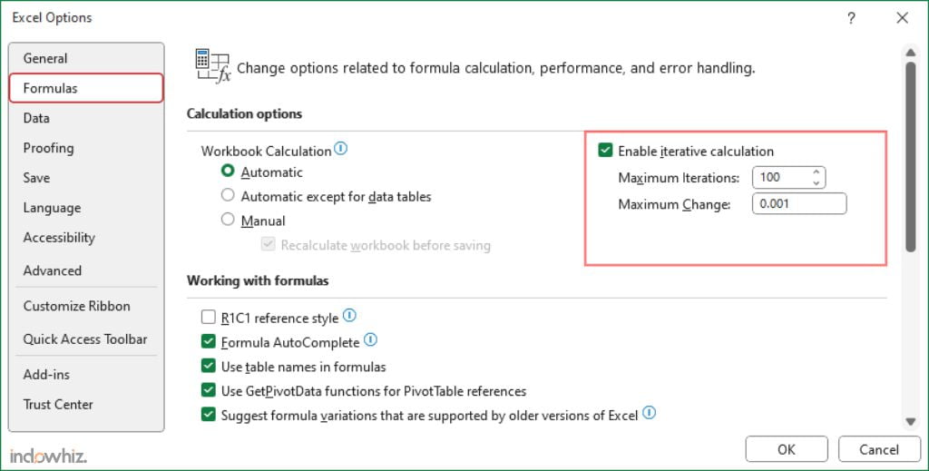
Several ways to fix #NUM! errors, such as:
- Evaluate your formula to locate the source of error.
If you have a complex formula, you may useError Checkingfeature. You can access this feature by going to theFormulastab and clicking theError Checkingbutton, or you can click the button near the error cell. Then, click onShow Calculation Steps. Then, evaluate your formula step by step to find where and why you got#NUM!
Ensure that your formula is valid and possible and that the value is within Excel’s capability. - Enable iterative calculation.
You may need to enable the iterative calculation in Excel, to use a function such asIRRorRATE, as in Figure 6. You can go toFile>Options. Then, on theFormulastab, underCalculation options, check theEnable iterative calculationbox. Then, clickOKto apply the changes. - Changing error display.
You can useIFERRORorIFfunctions to return an alternative error result instead of#NUM!. For example, using=IFERROR(SQRT(A2),“undefined”)will return an “undefined” string ifA2is negative.
7. #NULL!
There are different range operators to select cells, which can be used in a formula:
- Colon (:)
It separates thestart_cellandend_cellwhen you refer to a continuous range of cells. For example, a formula of=SUM(A1:A5)refers to the range that includes cellsA1throughA5. - Comma (,)
It is a union operator that combines two or more non-intersecting ranges or individual cells. For example,=SUM(A1:A5,C1:C5,D3,E3)refers to the union of the rangesA1:A5andC1:C5, and cellsD3andE3. - Space ( )
It is an intersection operator that returns the common cells between two or more ranges that intersect. For example,=SUM(A1:C3 B2:D4)refers to the intersection of the rangesA1:C3andB2:D4, which isB2:C3.
However, Excel will display #NULL! error if a formula contains an incorrect range operator, or contains a nonintersecting range while using space. For example, =SUM(A1 A10) will return #NULL! because there is no intersection between the ranges, or it is simply because of using space instead of a colon.
To fix a #NULL! error, you need to check your formula and make sure you use the correct range operator or intersection operator for your intended calculation. In addition, you can use the Error Checking feature in Excel to locate the source of the error. You can access it by going to the Formulas tab and clicking the Error Checking button, or you can click the button near the error cell. Then, click on Show Calculation Steps. Then, evaluate your formula step by step to find where and why you got #NULL!
8. #N/A
Excel displays #N/A error when a formula cannot find what it has been asked to look for. Commonly, it shows when you use XLOOKUP, VLOOKUP, HLOOKUP, LOOKUP, or MATCH functions, but the lookup value does not exist in the source data.
For example, as illustrated in Figure 7, “Pineapple” value does not exist in the source data (E2:F5). Therefore, VLOOKUP will return #N/A.
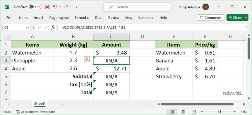
#N/A error due to a nonexistent value in the source dataSeveral ways to fix #N/A errors, such as:
- Evaluate your formula to locate the source of error.
If you have a complex formula, you may useError Checkingfeature. You can access this feature by going to theFormulastab and clicking theError Checkingbutton, or you can click the button near the error cell. Then, click onShow Calculation Steps. Then, evaluate your formula step by step to find where and why you got#N/Aerror. - Checking data types and extra space.
Make sure that the data types of the lookup value and the source data match. In addition, make sure that there are no extra spaces in the lookup value or the source data that may prevent a match. For example, if the lookup value is “Apple” with a trailing space, you can remove it using theTRIMfunction or theFind and Replacefeature. - Make sure to use the correct match type.
Make sure that you use the correct match type argument for your lookup function. For example,VLOOKUPhas the syntax of=VLOOKUP (lookup_value, table_array, col_index_num, [range_lookup]). Then, ifrange_lookupis set to be an approximate match (TRUEor1), you need to sort the source data in ascending order by the first column. Otherwise, if you use an exact match (FALSEor0), you do not need to sort the data. - Changing error display.
You can useIFERRORorIFfunctions to return an alternative error result instead of#N/AFor example, =IFERROR(VLOOKUP(A1,B1:C10,2,FALSE),“Not found”)will return “Not found” instead, ifVLOOKUPreturns#N/A.
9. #SPILL!
Excel 365, Excel 2021, and newer versions of Excel have dynamic arrays feature that allows formulas to return multiple results (as an array) and spill them into adjacent cells automatically.
However, Excel will show #SPILL! error if it cannot spill the results into adjacent cells, because they are occupied by other data or objects. This usually happens when you use a dynamic array function, such as FILTER, SORT, UNIQUE, SEQUENCE, or RANDARRAY, or any other formula that can produce an array of values.
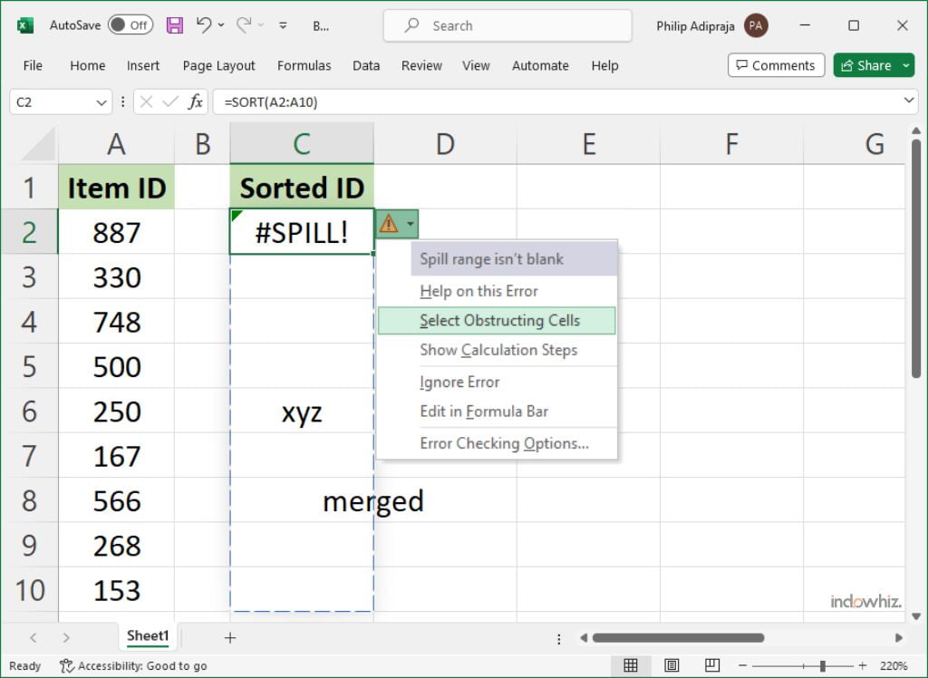
#SPILL!Several ways to fix #SPILL!
- Clearing the spill range.
You can select the Error floatie, and choose theSelect Obstructing Cellsoption to immediately go to the obstructing cell(s), as in Figure 8. Then, clear the cells by either deleting or moving the obstructing cell’s values. - Evaluate your formula to locate the source of error.
If you have a complex formula, you may useError Checkingfeature. You can access this feature by going to theFormulastab and clicking theError Checkingbutton, or you can click the button near the error cell. Then, click onShow Calculation Steps. Then, evaluate your formula step by step to find where and why you got#SPILL! - Use implicit intersection operator “@”.
You can try to add “implicit intersection” using the @ operator, and then copy the formula down. For example, if you add a formula of=VLOOKUP(@A:A,A:C,2,FALSE)in cellE2, then you need to copy the formula down until the end of the table (e.g., untilE10). In this case, it may return on one cell, not as a dynamic array.
10. #CALC!
Another type of error in a dynamic array, #CALC! is an error message when a formula encounters a calculation problem. There are several scenarios as the following and the way to address them.
- Empty array.
If a formula returns an empty array, such as when using theFILTERfunction with no matching criteria, Excel will display a#CALC!error. To avoid this, you need to specify a value for theif_emptyargument of the function, such as “NULL” or “=FILTER(C3:D5,D3:D5<100,"NULL")would return “NULL” if there are no items in the array. - Nested array or array of ranges.
Currently, Excel is unable to calculate an array within an array. Therefore, if a formula contains a nested array with more than one dimension, Excel will return#CALC!error. For example, Excel is able to calculate=MUNIT(2), but unable to calculate=MUNIT({1,2}). Therefore, make sure that you avoid using a nested array or array of ranges. - Too many cells.
If you are using Excel for web, the#CALC!error may occur when a function refers to more than10,000cells. However, the desktop version of Excel does not have this limitation (or simply has a far higher limit). - Incorrect
LAMBDAusage.
When you useLAMBDAfunction in a cell, you must assign it with the reference cells. Otherwise, it will return#CALC!error. For example,=LAMBDA(x,y, x+y)will return#CALC!error, because has no references. However, if you add the references with the right argument, such as=LAMBDA(x,y, x+y)(A1, B1), the function will run smoothly.
In addition, you can use the Error Checking feature in Excel to locate the source of error. You can access it by going to the Formulas tab and clicking the Error Checking button, or you can click the button near the error cell. Then, click on Show Calculation Steps. Then, evaluate your formula step by step to find where and why you got #CALC!
11. Circular reference error
A circular reference in Excel is a type of error that occurs when a formula in a cell refers to itself directly or indirectly. By default, this creates iterations that prevent Excel from calculating the formula correctly. Then, Excel will return 0 (zero) by default.
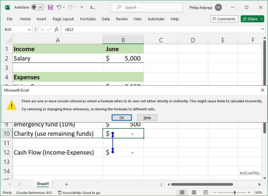
For example, if cell A1 contains the formula =A1+1, this is a direct circular reference because the formula refers to the same cell. On the other hand, If cell A1 contains the formula =B1+1 and cell B1 contains the formula =A1+1, it will create an indirect circular reference because the formula refers to another cell that refers back to the original cell. Usually, for indirect circular reference, you will see a blue arrow pointing back to the same cell or forming a loop with other cells, as in Figure 9.
There are different ways to fix circular references in Excel, such as:
- Enable iterative calculation.
If you want to calculate the iteration of the circular references, you can enable the iterative calculation option, as in Figure 6. You can go toFile>Options. Then, on theFormulastab, underCalculation options, check theEnable iterative calculationbox. Then, clickOKto apply the changes. - Edit your formula.
If you accidentally get a circular reference error, you may need to edit or delete the formula that causes it. You can check the syntax and logic of your formula and make sure it does not refer to itself or another cell that refers back to it.
