Last Updated on October 30, 2020
Linear Regression with Gradient Descent is a good and simple method for time series prediction. One of the time series predictions that can be solved by this method is Energy Efficiency Prediction. And the purpose of this research article is to implement Linear Regression with Gradient Descent to predict the Heating Load (Y1). The programming language used for this case is using Python code. The data can be downloaded from https://archive.ics.uci.edu/ml/datasets/Energy+efficiency.
The training data used 50% from the dataset and testing data also used 50% from the dataset. The dataset has eight input data there is Relative Compactness (X1), Surface Area (X2), Wall Area (X3), Roof Area (X4), Overall Height (X5), Orientation (X6), Glazing Area (X7), and Glazing Area (X8). This article will show a brief discussion of prediction results using Linear Regression with Gradient Descent.
DEVELOPMENT
Gradient Descent comes with some procedure that is:
- Procedure
- Start with random values
-
- Slightly move
to reduce
- Keep doing step 2 until converges
- Start with random values
Technologies Used
To solve this problem, it was used the Python 3 language with the following libraries:
- Pandas: Python library for data structures and statistical tools (McKinney, 2010).
- Numpy: The Python libraries for the base data structure used for data and model parameters were presented as Numpy arrays (Al-Shalabi et al., 2006).
- Sklearn (Hunter, 2007).
IMPLEMENTATION USING PYTHON CODE
The python code in all of this article could be merged into a single python file (e.g. gdescent.py). However, you may need to convert the data from ENB2012_data.xlsx into ENB2012_data.csv, by using spreadsheet software such as Excel or similar.
Import libraries:
import sys

import numpy
import pandas
import sklearn.metrics
import sklearn.model_selection
import sklearn.linear_model
import sklearn.preprocessing
Loading Dataset:
def load_train_test_data(train_ratio=.5):
    data = pandas.read_csv('./ENB2012_data.csv')

    feature_col = ['X1', 'X2', 'X3', 'X4', 'X5', 'X6', 'X7', 'X8']
    label_col = ['Y1']
    X = data[feature_col]
    y = data[label_col]

    return sklearn.model_selection.train_test_split(X, y, test_size = 1 - train_ratio, random_state=0)
Scale the Training and Testing Features
def scale_features(X_train, X_test, low=0, upp=1):
    minmax_scaler = sklearn.preprocessing.MinMaxScaler(feature_range=(low, upp)).fit(numpy.vstack((X_train, X_test)))
    X_train_scale = minmax_scaler.transform(X_train)
    X_test_scale = minmax_scaler.transform(X_test)
    return X_train_scale, X_test_scale
Gradient Descent Calculation
def gradient_descent(X, y, alpha=0.1, iters=100000, eps=1e-4):
    n, d = X.shape
    theta = numpy.zeros((d, 1))
    xT = numpy.transpose(X)

    for k in range(1,iters+1):
        theta_k = theta.copy()
        prediction = numpy.dot(X,theta)
        error = numpy.subtract(prediction,y)
        #gradient
        gradient = numpy.dot(xT,error) * (1/n)
        #update theta
        theta = theta_k - (alpha * gradient)
        print(k)

    for delta in abs(theta-theta_k):
        if delta > eps:
            break

    return theta
Prediction Function
def predict(X, theta):
    return numpy.dot(X, theta)
Main Function
def main(argv):
    X_train, X_test, y_train, y_test = load_train_test_data(train_ratio=.5)
    X_train_scale, X_test_scale = scale_features(X_train, X_test, 0, 1)

    theta = gradient_descent(X_train_scale, y_train)
    print('Theta:\n', theta)

    y_hat = predict(X_train_scale, theta)
    print("Linear train R^2: %f" % (sklearn.metrics.r2_score(y_train, y_hat)))
    y_hat = predict(X_test_scale, theta)
    #R2 value closer to 1 indicating that a greater proportion of variance is accounted for by the model.
    print("Linear test R^2: %f" % (sklearn.metrics.r2_score(y_test, y_hat)))

    #MSE value closer to 0 indicates a fit that is more useful for prediction.
    print("Mean Squared Error Test : %f" % (sklearn.metrics.mean_squared_error(y_test, y_hat)))
    print("Mean Absolute Error Test : %f" % (sklearn.metrics.mean_absolute_error(y_test, y_hat)))

if __name__ == "__main__":
    main(sys.argv)
RESULT AND DISCUSSION
This article shows the result of the experiment using some parameter value there is the value of alpha and maximum iteration. this experiment is aiming to find the optimum parameter value to predict the Heating Load (Y1).
Testing Value of Alpha
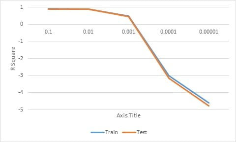
The process of testing the value of alpha was done one time, the value of alpha was 0.1 to 0.000001. The values of maximum iteration used constantly that is 1000. The optimum value of alpha can be seen from the R2 result. The test results on the R2 value shown in Table 1. The chart of R2 value changes according to the value of alpha can be seen in Figure 1.
Table 1. R2 value from Testing Value of Alpha
| Value of Alpha | R Square | |
| Train | Test | |
| 0.1 | 0.920143 | 0.896159 |
| 0.01 | 0.903376 | 0.880996 |
| 0.001 | 0.496769 | 0.460076 |
| 0.0001 | -2.993605 | -3.154529 |
| 0.00001 | -4.593513 | -4.765798 |
The testing results value of alpha in Table 1 indicates that the best R2 value was obtained with value of alpha is 0.1.


Testing Value of Maximum Iteration
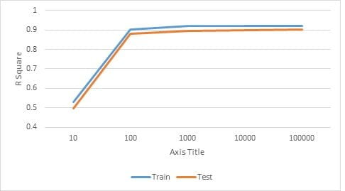
The process of testing the value of Maximum Iteration was done one time, the value of Maximum Iteration was 10 to 10000. The values of alpha used from the previous testing that is 0.1. The optimum value of Maximum Iteration can be seen from the R2 result. The test results on the R2 value shown in Table 2. The chart of R2 value changes according to the value of Maximum Iteration can be seen in Figure 2.
Table 2. R2 value from Testing Value of Maximum Iteration
| Value of Max Iteration | R Square | |
| Train | Test | |
| 10 | 0.529225 | 0.497496 |
| 100 | 0.903513 | 0.881109 |
| 1000 | 0.920143 | 0.896159 |
| 10000 | 0.921027 | 0.900045 |
| 100000 | 0.92156 | 0.900637 |
The testing results value of Maximum Iteration in Table 2 indicate that the best R2 value was obtained with a value of Maximum Iteration is 10000. Because of that, I choose maximum iteration at 10,000 because after that nothing significant improvement of R2 value. So, the optimum maximum generation is 10,000 because it also considers the value running time.

Result Analysis
We can see from Figure 2, the R2 value accuracy from training data at the blue line and the R2 value from testing data at the orange line. From the testing and training data, the optimal value of alpha is 0.1 and the optimum maximum iteration is 10000. Form the testing parameter value, Linear regression using Gradient Descent can predict the Heating Load (Y1) with R2 value 0.92156 for training and 0.900637 for testing. The detail result form this experiment can see in the figure below:
Theta:
 [[ 2.32952123]
 [ 2.97557991]
 [ 8.4017958 ]
 [19.42200572]
 [-0.32337598]
 [ 7.52095841]
 [ 0.86006606]]
Linear train R^2: 0.921027
Linear test R^2: 0.900045
Mean Squared Error Test : 10.275206
Mean Absolute Error Test : 2.369451
So we can write the formulation to find Heating Load (Y1) as follow:
Read Also: Implementation of K-Nearest Neighbors (KNN) For Iris Classification Using Python 3
REFERENCES
Al-Shalabi, R., Kanaan, G., & Gharaibeh, M. H. (2006). Arabic Text Categorization Using kNN Algorithm. Proceedings of The 4th International Multiconference on Computer Science and Information Technology, 5–7.
Hunter, J. D. (2007). Matplotlib: A 2D Graphics Environment. Computing in Science & Engineering, 9(3), 90–95. https://doi.org/10.1109/MCSE.2007.55
Lotte, F., Congedo, M., Lécuyer, A., Lamarche, F., & Arnaldi, B. (2007). A review of classification algorithms for EEG-based brain-computer interfaces. Journal of Neural Engineering, 4(2). https://doi.org/10.1088/1741-2560/4/2/R01
McKinney, W. (2010). Data Structures for Statistical Computing in Python. Proceedings of the 9th Python in Science Conference, 1697900(Scipy), 51–56. Retrieved from http://conference.scipy.org/proceedings/scipy2010/mckinney.html
Featured Image Source: Freepik
Appendix
The full code:
import sys

import numpy
import pandas
import sklearn.metrics
import sklearn.model_selection
import sklearn.linear_model
import sklearn.preprocessing

def load_train_test_data(train_ratio=.5):
    data = pandas.read_csv('./ENB2012_data.csv')

    feature_col = ['X1', 'X2', 'X3', 'X4', 'X5', 'X6', 'X7', 'X8']
    label_col = ['Y1']
    X = data[feature_col]
    y = data[label_col]

    return sklearn.model_selection.train_test_split(X, y, test_size = 1 - train_ratio, random_state=0)

def scale_features(X_train, X_test, low=0, upp=1):
    minmax_scaler = sklearn.preprocessing.MinMaxScaler(feature_range=(low, upp)).fit(numpy.vstack((X_train, X_test)))
    X_train_scale = minmax_scaler.transform(X_train)
    X_test_scale = minmax_scaler.transform(X_test)
    return X_train_scale, X_test_scale

def gradient_descent(X, y, alpha=0.1, iters=100000, eps=1e-4):
    n, d = X.shape
    theta = numpy.zeros((d, 1))
    xT = numpy.transpose(X)

    for k in range(1,iters+1):
        theta_k = theta.copy()
        prediction = numpy.dot(X,theta)
        error = numpy.subtract(prediction,y)
        #gradient
        gradient = numpy.dot(xT,error) * (1/n)
        #update theta
        theta = theta_k - (alpha * gradient)
        print(k)

    for delta in abs(theta-theta_k):
        if delta > eps:
            break

    return theta

def predict(X, theta):
    return numpy.dot(X, theta)

def main(argv):
    X_train, X_test, y_train, y_test = load_train_test_data(train_ratio=.5)
    X_train_scale, X_test_scale = scale_features(X_train, X_test, 0, 1)

    theta = gradient_descent(X_train_scale, y_train)
    print('Theta:\n', theta)

    y_hat = predict(X_train_scale, theta)
    print("Linear train R^2: %f" % (sklearn.metrics.r2_score(y_train, y_hat)))
    y_hat = predict(X_test_scale, theta)
    #R2 value closer to 1 indicating that a greater proportion of variance is accounted for by the model.
    print("Linear test R^2: %f" % (sklearn.metrics.r2_score(y_test, y_hat)))

    #MSE value closer to 0 indicates a fit that is more useful for prediction.
    print("Mean Squared Error Test : %f" % (sklearn.metrics.mean_squared_error(y_test, y_hat)))
    print("Mean Absolute Error Test : %f" % (sklearn.metrics.mean_absolute_error(y_test, y_hat)))

if __name__ == "__main__":
    main(sys.argv)


Hello, may I request your source code to study? Thank you very much! Your article is very great!
We already update the article, so you could find the full code from the appendix.
however, because we use read_csv function, you may require to convert the training data from xlsx into csv.